IBMPopSim C++ essentials

The arguments intensity_code, interaction_code and kernel_code of the events functions must contain some C++ code given by the user. You don’t need to be a C++ guru to write the few instructions needed. These functions should use very little C++ syntax. They are essentially arithmetic or logical operations, tests and calls to predefined functions, which we give an overview below.

For code efficiency, you should not allocate memory in these functions (no new) or use type containers (std::vector, std::list, …). If you think you need to allocate memory, consider as parameter an R vector that will be mapped via arma::vector (see below), or declare the variable as static. Also, it should not be necessary to make a loop. Keep in mind that these functions should be fast.

There are no C++ language restrictions so you can use all the functions of the standard C++11 library. However we detail in this section some functions that should be sufficient. For more details on C++ and Rcpp we recommend:

C++ syntax

Each statement must be ended by a semicolon.
Single-line comments start with two forward slashes //.
To create a variable, you must specify the type and assign it a value (type variable = value;). Here some examples:

int myNum = 5;               // Integer (whole number without decimals)
double myFloatNum = 5.99;    // Floating point number (with decimals)
char myLetter = 'D';         // Character
bool myBoolean = true;       // Boolean (true or false)

bool data type can take the values true (1) or false (0).
C++ supports the usual logical conditions from mathematics:
- Less than: a < b
- Less than or equal to: a <= b
- Greater than: a > b
- Greater than or equal to: a >= b
- Equal to a == b
- Not Equal to: a != b
The logical operators are: !, &&, ||
The arithmetic operators are: +, -, *, /, %
Compound assignment: +=, -=, *=, /=, %=
Increment and decrement: ++, --
Conditional ternary operator: ? : The conditional operator evaluates an expression, returning one value if that expression evaluates to true, and a different one if the expression evaluates as false. Its syntax is:

condition ? result1; : result2;

Use the if, else if, else statements to specify a block of C++ code to be executed if one or more conditions are or not true.

if (condition1) {
  // block of code to be executed if condition1 is true
} else if (condition2) {
  // block of code to be executed if the condition1 is false and condition2 is true
} else {
  // block of code to be executed if the condition1 is false and condition2 is false
}

The syntax of the switch statement is a bit peculiar. Its purpose is to check for a value among a number of possible constant expressions. It is something similar to concatenating if-else statements, but limited to constant expressions. Its most typical syntax is:

switch (expression)
{
  case constant1:
     group-of-statements-1;
     break;
  case constant2:
     group-of-statements-2;
     break;
  .
  .
  .
  default:
     default-group-of-statements
}

It works in the following way: switch evaluates expression and checks if it is equivalent to constant1; if it is, it executes group-of-statements-1 until it finds the break statement. When it finds this break statement, the program jumps to the end of the entire switch statement (the closing brace).

When you know exactly how many times you want to loop through a block of code, use the for loop.

for (statement 1; statement 2; statement 3) {
  // code block to be executed
}

The while loop loops through a block of code as long as a specified condition is true.

while (condition) {
  // code block to be executed
}

For more details we recommend a few pages of www.cplusplus.com about:

Usual numeric functions

The most popular functions of the cmath library, which is included in the package, are the following:

Exponential and logarithm functions: exp(x), log(x) (natural logarithm)
Trigonometric functions: cos(x), sin(x), tan(x)
Power functions: pow(x, a) meaning $x^a$ and sqrt(x) meaning $\sqrt{x}$
Absolute value: abs(x)
Truncation functions: ceil(x) meaning $\lceil x \rceil$ and floor(x) meaning $\lfloor x \rfloor$
Bivariate functions: max(x, y) and min(x,y)

Note that these functions are not vectorial, the arguments x and y must be scalar. If the user wants to call some other functions of cmath not listed in the table, this is possible by adding the prefix std:: to the name of the function (scope resolution operator :: to access to functions declared in namespace standard std).

Individuals characteristics and model parameters: link between R and C++

To facilitate the model creation, the individuals’ characteristics and a list model parameters can be declared in the R environment and used in the C++ code.

The data shared between the R environment and the C++ code are:

The characteristics of the individuals which must be atomic (Boolean, scalar or character).
The model parameters: a list of variables of type:
- Atomic, vector or matrix.
- Predefined real functions of one variable, or list of such functions.
- Piecewise real function of two variables, of list of such.

Atomic types (characteristics and parameters)

Here is the conversion table used between the atomic types of R and C++.

C++ type	R type
bool	`logical`
int	`integer`
double	`double`
char	`character`

Individuals characteristics

The characteristics of an individual are defined by a named character vector containing the name of the characteristic and the associated C++ type. The function ?get_characteristics provides a way to extract the characteristics from a population data frame.

library(IBMPopSim)
pop <- population(IBMPopSim::EW_popIMD_14$sample)
get_characteristics(pop)
##   male    IMD 
## "bool"  "int"

The requires birth and death characteristics are of type double.

Atomic model parameters

The model parameters are given by a named list of R objects. We recall that the type of an R object can be determined by calling the ?typeof function. Atomic objects declared as model parameters can be directly used in the C++ code.
In the example below, the variable code contains simple C++ instructions depending on the parameters defined in params. The summary of the model mod gives useful information on the types of characteristics and parameters used in C++ code.

params <- list("lambda" = 0.02, "alpha" = 0.4, "mu" = as.integer(2))
code <- "result = lambda + alpha * (age(I, t) + mu);"
event_birth <- mk_event_individual("birth", intensity_code = code)
mod <- mk_model(get_characteristics(pop), events = list("birth" = event_birth), 
                parameters = params, with_compilation = FALSE)
summary(mod)
## Events description:
## [[1]]    
## Event class : individual 
## Event type : birth 
## Event name : birth
## Intensity code : 'result = lambda + alpha * (age(I, t) + mu);' 
## Kernel code : '' 
## 
## --------------------------------------- 
## Individual description:
## names:  birth death male IMD 
## R types:  double double logical integer 
## C types:  double double bool int 
## --------------------------------------- 
## R parameters available in C++ code:
## names:  lambda alpha mu 
## R types:  double double integer 
## C types:  double double int

Vectors and matrices (model parameters)

Two of the possible model parameters types given in the argument parameters of the ?mk_model function are R vectors and R matrices. We call R vector a numeric of length at least 2. These types are converted, using the RcppArmadillo library, in C++ Armadillo types, arma::vec and arma::matrix respectively.

The classes arma::vec and arma::matrix are rich and easy-to-use implementations of one-dimensional and two-dimensional arrays. To access to individual elements of an array, use the operator () (or [] in dimension 1).

(n) or [n] for arma::vec, access the n-th element.
(i,j) for arma::matrix, access the element stored at the $i$-th row and $j$-th column.

Warning: The first element of the array is indexed by subscript of 0 (in each dimension).

Another standard way (in C++) to access elements is to used iterators. An iterator is an object that, pointing to some element in a range of elements, has the ability to iterate through the elements of that range using a set of operators (see more details on iterators).

Let v be a an object of type arma::vec and A be a an object of type arma::matrix. Here we show how to get the begin and the end iterators of these objects.

v.begin(): iterator pointing to the begin of v
v.end(): iterator pointing to the end of v
A.begin_row(i): iterator pointing to the first element of row i
A.end_row(i): iterator pointing to the last element of row i
A.begin_col(i): iterator pointing to the first element of column i
A.end_col(i): iterator pointing to the last element of column i

Predefined functions (model parameters)

To facilitate the implementation of intensity functions and kernel code, R functions have been predefined in IBMPopSim, which can be defined as model parameters and then called in the C++ code. The goal is to make their use as transparent as possible.

Real functions of one variable

Here is a list of such functions that can be defined as a R object and called from R and C++.

stepfun: Step function.
linfun: Linear interpolation function.
gompertz: Gompertz–Makeham intensity function.
weibull: Weibull density function.
piecewise_x: Piecewise real function.

See the reference manual for mathematical definitions of these functions (?stepfun).
Once the model is created, these predefined functions are transformed into C++ functions, identified as function_x.

We illustrate below some examples of the use of these functions:

We define dr a stepfun depending on some values in EW_pop_14$rates. Note that this function applies to an age a.

library(ggfortify)
dr <- with(EW_pop_14$rates,
           stepfun(x = death_male[,"age"], y = c(0, death_male[,"value"])))
autoplot(dr, xlab="age", ylab="dr", shape=NULL,main="Example of step function")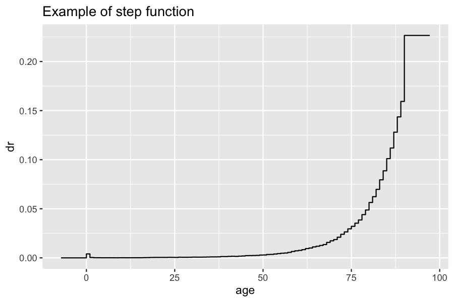

We can also initialize a piecewise real function f defined by the function dr before age 80, and by a Gompertz-Makeham intensity function for ages after 80.

f <- piecewise_x(80, list(dr, gompertz(0.00006, 0.085)))
x <- seq(40, 110)
ggplot(data.frame(x=x, y=sapply(x, f)), aes(x=x, y=y))+ geom_step() + xlab("Age") +ylab("f") + ggtitle("Example of piecewise function")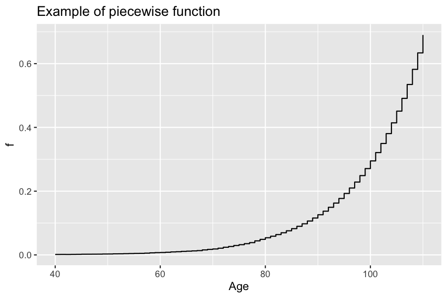

Once a function has been created and defined as model parameter, a model depending on the function can be defined. For example we use in the model below the stepfun dr as a model parameter named rate. The function is used to defined the intensity of death events in the model. s

params <- list("rate" = dr)
event <- mk_event_individual("death", intensity_code = "result = rate(age(I, t));")
mod <- mk_model(get_characteristics(pop), events = list("death" = event), 
                parameters = params, with_compilation = FALSE)
summary(mod)
## Events description:
## [[1]]    
## Event class : individual 
## Event type : death 
## Event name : death
## Intensity code : 'result = rate(age(I, t));' 
## Kernel code : '' 
## 
## --------------------------------------- 
## Individual description:
## names:  birth death male IMD 
## R types:  double double logical integer 
## C types:  double double bool int 
## --------------------------------------- 
## R parameters available in C++ code:
## names:  rate 
## R types:  closure 
## C types:  function_x

After compilation, the parameter rate can actually be replaced by any function of type function_x. For example you can call

popsim(mod, pop, params = list("rate" = dr), age_max = 120, 
       events_bounds = c("death" = dr(age_max)), time = 10)

as well as

popsim(mod, pop, params = list("rate" = f), age_max = 120, 
       events_bounds = c("death" = f(age_max)), time = 10)

Piecewise real functions of two variables

In the C++ code these R functions declared with ?piecewise_xy are identified as function_xy functions. See ?piecewise_xy for mathematical definition. This function allows to easily define a step function that depend on age and time.

List of functions

As parameter you can use a list of functions. All R functions in the list must be of the same C++ type: either function_x or function_xy. In C++ code the list of functions is replaced by a std::vector of function_x or function_xy (with first element indexed by 0).

Random variables

We use the following notations to describe the available C++ random distributions, which can be used in the C++ intensity and kernel codes.

$\mathcal{U}(a,b)$ : Uniform distribution on $[a, b]$ with $a < b$
$\mathcal{E}(\lambda)$ : Exponential distribution, $\lambda > 0$
$\mathcal{N}(\mu,\sigma)$ : Gaussian distribution, $\mu, \sigma \in \mathbf{R}$
$\mathrm{Pois}(\lambda)$: Poisson distribution, $\lambda > 0$
$\Gamma(\alpha, \beta)$: Gamma distribution, $\alpha > 0$, $\beta > 0$
$\mathrm{Weib}(a, b)$: Weibull distribution, $a > 0$, $b > 0$
$\mathcal{U}\{a, b\}$: Discrete uniform distribution on $\{a, a+1, \dots, b\}$ with $a < b$
$\mathcal{B}(p)$: Bernoulli distribution, the probability of success is $p \in (0,1)$
$\mathcal{B}(n, p)$: Binomial distribution $n \ge 1$, $p \in (0,1)$
$\mathcal{D}_n$ : Discrete distribution with values in $\{ 0, \dots, n-1 \}$ and with probabilities $\{p_0, \dots, p_{n-1}\}$.

In the table below we show how to call them, which means how to make independent realizations of these random variables, and we give the reference to the C++ corresponding function of the random library hidden in this call.

Function call	Meaning	C++ `random` internal function
CUnif($a=0, b=1$)	$\mathcal{U}(a,b)$	`uniform_real_distribution<double>`
CExp($\lambda=1$)	$\mathcal{E}(\lambda)$	`exponential_distribution<double>`
CNorm($\mu=0, \sigma=1$)	$\mathcal{N}(\mu,\sigma)$	`normal_distribution<double>`
CPoisson($\lambda=1$)	$\mathrm{Pois}(\lambda)$	`poisson_distribution<unsigned>`
CGamma($\alpha=1, \beta=1$)	$\Gamma(\alpha,\beta)$	`gamma_distribution<double>`
CWeibull($a=1$, $b=1$)	$\mathrm{Weib}(a,b)$	`weibull_distribution<double>`
CUnifInt($a=0, b=2^{31}-1$)	$\mathcal{U}\{a,b\}$	`uniform_int_distribution<int>`
CBern($p=0.5$)	$\mathcal{B}(p)$	`bernoulli_distribution`
CBinom($n=1, p=0.5$)	$\mathcal{B}(n,p)$	`binomial_distribution<int>`
CDiscrete(`p_begin`, `p_end`)	$\mathcal{D}_n$	`discrete_distribution<int>`

In the discrete distribution call CDiscrete(p_begin, p_end), the arguments p_begin and p_end represent the iterators to the begin and to the end of an array which contains $\{p_0, \dots, p_{n-1}\}$. Note that the use of iterators is a convenient and fast way to access a column or row of a matrix arma::mat.

Function call	Meaning	C++ `random` internal function
CUnif(\(a=0, b=1\))	\(\mathcal{U}(a,b)\)	`uniform_real_distribution<double>`
CExp(\(\lambda=1\))	\(\mathcal{E}(\lambda)\)	`exponential_distribution<double>`
CNorm(\(\mu=0, \sigma=1\))	\(\mathcal{N}(\mu,\sigma)\)	`normal_distribution<double>`
CPoisson(\(\lambda=1\))	\(\mathrm{Pois}(\lambda)\)	`poisson_distribution<unsigned>`
CGamma(\(\alpha=1, \beta=1\))	\(\Gamma(\alpha,\beta)\)	`gamma_distribution<double>`
CWeibull(\(a=1\), \(b=1\))	\(\mathrm{Weib}(a,b)\)	`weibull_distribution<double>`
CUnifInt(\(a=0, b=2^{31}-1\))	\(\mathcal{U}\{a,b\}\)	`uniform_int_distribution<int>`
CBern(\(p=0.5\))	\(\mathcal{B}(p)\)	`bernoulli_distribution`
CBinom(\(n=1, p=0.5\))	\(\mathcal{B}(n,p)\)	`binomial_distribution<int>`
CDiscrete(`p_begin`, `p_end`)	\(\mathcal{D}_n\)	`discrete_distribution<int>`

Daphné Giorgi, Sarah Kaakai, Vincent Lemaire